Texture Synthesis and Hole-Filling
How do we cut something out of an image, and fill the hole naturally?
Definition Texture depicts spacially repeating patterns.
Texture Synthesis
Create new samples of a given texture. Many applications: virtual environments, hole-filling, texturing surfaces.
The challenge:
Need to model the whole spectrum: from repeated to stochastic texture.
One idea:
- Compute statistics of input texture
- Generate a new texture that keeps those same statistics.
But it is hard to model those probabilities distributions.
Another idea: ==Efros & Leung algorithm==
Given the neighbour, we want to calculate the probabiliy of appearing this pixel $p$ in the middle.
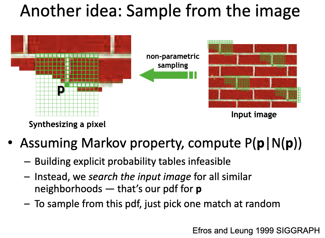
How to match pixels?
- Gaussian-weighted SSD (sum square difference) gives us more emphasis on nearby pixels.
\begin{align*} \text{SSD}(P, Q) = \sum_{i, j}(p_{ij} - q_{ij})^2 w_{ij}\\ \text{where } w_{ij} = e^{ \frac{-(1-w/2)^2 - (j - h/2)^2}{2 \sigma^2} } \end{align*}
where $P$, and $Q$, are two patches, $w$ and $h$ in the $w_{ij}$ is the width and height of the patch.
-
What order to fill in new pixels?
- “Onion skin” order: pixels with most neighbors are synthesized first.
How big should the patches be? The size of neighborhood window decides how stochasticity of the texture. A smaller window size gives a more random output.
Texture synthesis algorithm
While image not filled:
- Get unfilled pixels with filled neighbors, sorted by the numebr of filled neighbors. (priority queue?)
- For each pixel, get top N matches based on visible neighbors. This is where we use the Gaussian-weighted SSD.
- Randomly select one of the matches and copy pixels from it.
This algorithm can be used for hole filling, extrapolation, …
Hole-Filling
We can just use the texture synthesis algorithm.BUT, the order of filling matters.

Sometimes, we can add more weights for the continuous edges when peforming the onion filling. (Gradient sensitive). It makes the edges to be more intact.
We want it to be faster
The Efros & Leung texture synthesis algorithm is simple and good, but too slow…
The next iteration is: Image quilting (Efros & Freeman 2001).
It depends on the observation that: neighbor pixels are highly correlated. Now, instead of filling pixel by pixel, we fill block by block.
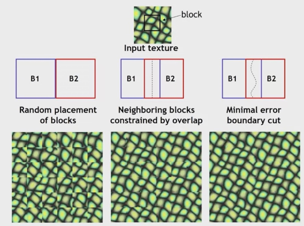
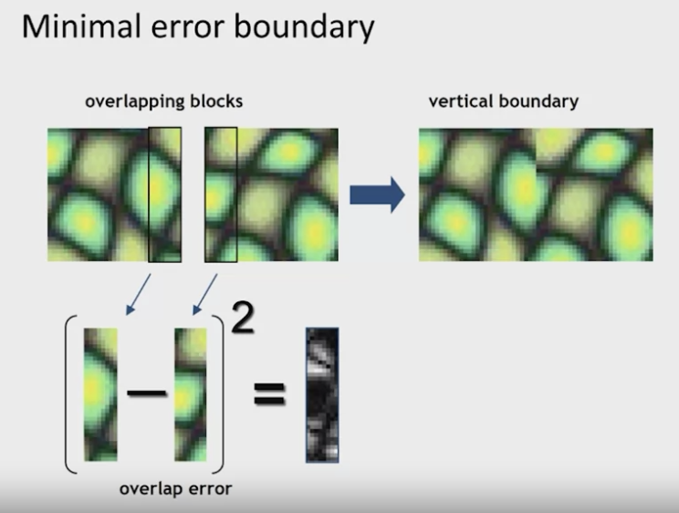
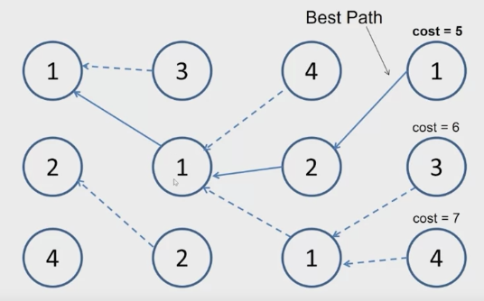
We need to put the tiles together. To make them look seemless, we can use this minimal error boundary cut. We calculate the square difference of the overlapping part, and calcualte the boundary. Using this simplified Dijikstra’s algorithm, we can easy calculate what we want.
Texture Transfer
Very similar to texture synthesis, but in a more restricted condition: $$ \text{cost} = \alpha * \text{SSD}{overlap} + (1-\alpha)* \text{SSD}{transfer} $$
Image Analogies
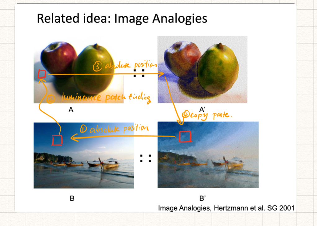
Intelligent Scissors and Graph Cuts
We want to find seams and boundaries. Then, CUT!
Fundamental Concepts: The image as a Graph
- Intelligent Scissers: Good boundary = short path
- Graph cuts: Good region has low cutting cost.
The goal ofSemi-automated segmentation: User provides imprecise and incomplete specification of region — your algorithm has to read his/her mind.
A good region:
- Contains small range of color/ texture.
- Looks different than background
- Compact
A good boundary:
- High gradient along boundary
- Gradient in right direction
- Smooth
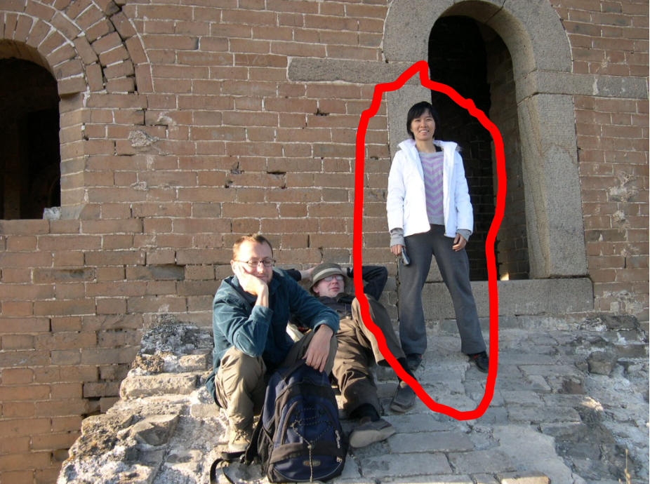
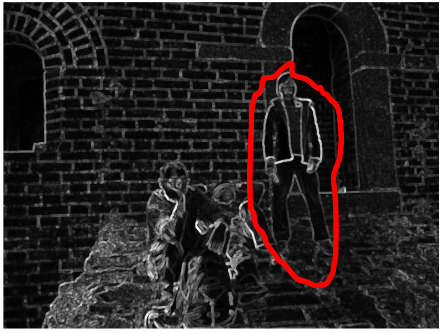
Intelligent Scissors
Consider these image as a graph. Think of pixels as nodes, and think of cost of the path between two pixels as weighted edges.
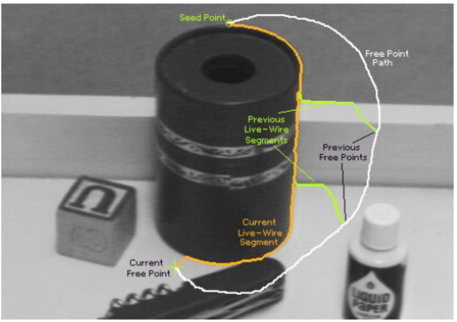
Formulation: find good boundary between seed points.
Challenges:
- Minimize interaction time
- Define what makes a good boundary
- Efficienctly find it
Luckily, these can be achieved by using Dijkstra’s algorithm with a properly defined graph.
Intelligent Scissors method
-
Define boundary cost between neighboring pixels
-
Lower if edge is present
-
Lower is gradient is strong
-
Lower if gradient is in direction of boundary
-
-
User specifies a starting point (seed)
- A little snapping to the edges makes pixel-perfect operation not neccessary.
-
Compute lowest cost from seed to each other pixel
- Dijkstra’s shortest path algorithm
-
Get path from seed to cursor, choose new seed, repeat
Using this boundary cost, the path tends to follow the edges of objects. It makes the algorithm works. Dijkstra’s algorithm makes it fast.
Graph Cuts
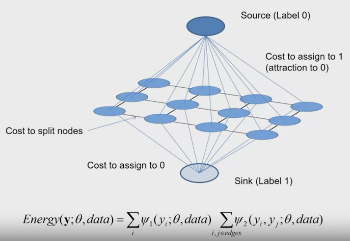
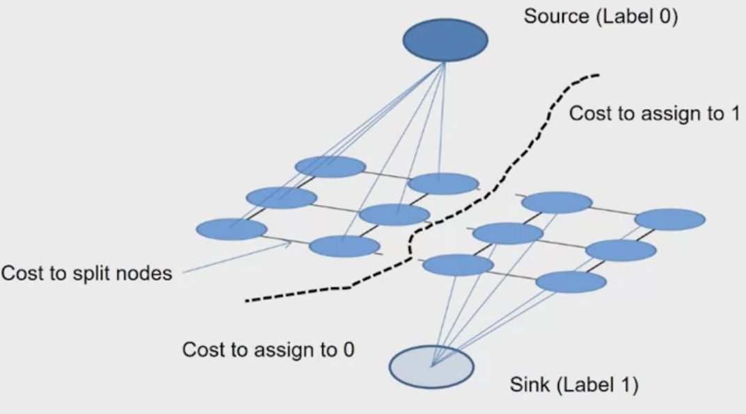
Look at the energe function, $y$ in the function represents the label of pixels (whether they belong to label 0 or 1). And, there are two kinds of cost.
- The first one is the unary cost, it measures whether the pixel is more similar to label 0 or 1.
- The second one is a pair wise cose, which allows groups of pixels to be assigned to the same label.
The goal of the graph cut algorithm is to find a cut through the graph to seperate the foreground and the background.
The Graph Cut Segmentation algorithm:
- Define graph
- usually 4-connected or 8-connected
- Set weights to foreground/background
- Color histogram or mixture of Gaussians for background and foreground. More foreground tends to be negative.
$$ \textit { unary_ potential }(x)=-\log \left(\frac{P\left(c(x) ; \theta_{\text {foreground }}\right)}{P\left(c(x) ; \theta_{\text {background }}\right)}\right) $$ 3. Set weights for edges between pixels
$$ \textit { edge_ potential }(x, y)=k_1+k_2 \exp\left{ \frac{-|c(x)-c(y)|^2}{2 \sigma^2} \right} $$
- Apply min-cut/max-flow algorithm foreground, background models
- Return to 2, using current labels to compute foreground, background models.
Limitations of Graph Cut
- Requires associative graphs
- Connected notes should prefer to have the same label
- Is optimal only for binary problems
Reference
CS445 Derek Hoiem: https://courses.engr.illinois.edu/cs445/fa2023/